What Can Crack Images Tell Us About Their Behaviour?
Abijeet Rajasekaran · Aditya Kaleeswar
While working on CRAFT, we had a vision component that identified cracks and other visual hazards (for example, fire, cracks, and smoke). That made sense for a rover exploring a space: find something worth inspecting, record its location, and add it to the map. But a crack detection left me with another question. What could we actually say about the crack after finding it?
Looking at pretrained models and crack datasets made that question harder to ignore. A model could pick out a thin surface trace quite convincingly. Its mask could look good. But that did not tell us whether the crack mattered structurally, or how it might behave under a load. That became the starting point for this project: could we take the output of a vision model, turn it into useful measurements, and connect those measurements to a mechanics model? This post follows how we approached that question, from choosing a manageable fracture problem to designing the CV pipeline around the inputs it needed. The PINN is part of the larger project; here, I want to explain how we get to the point where its inputs mean something.
The question behind the width threshold
One of the things we looked into was guidance on acceptable crack widths. It is tempting to turn that into a simple rule: below some width, a crack is cosmetic; above it, the crack is dangerous. The references need a more careful reading. ACI’s discussion of ACI 224R-01 describes reasonable crack widths under service loads and notes that widths vary and can change over time. It does not establish a universal width that separates safe structures from unsafe ones. ACI’s explanation. An ACI symposium paper reproduces the exposure-dependent guidance: for example, 0.30 mm for humidity, moist air, or soil, and 0.15 mm for seawater. Those are different conditions, not two competing definitions of structural failure. Patnaik et al., Reduction of Crack Width with Fiber. For our project, the useful question became: what information is missing when all we have is a visible crack and its width?
We need to know the geometry we are analysing, the load acting on it, and the material’s resistance to fracture. We also need to know whether our chosen model describes that situation at all. A narrow-looking line in a photograph cannot supply those answers by itself. There is a practical detail here worth being open about. The existing prototype contains a 0.3 mm width filter with an overly broad “non-structural” label. I would not treat that label as an engineering conclusion. The length-validation experiments disable the width filter; the results later in this post do not depend on classifying thin cracks as harmless.
How would this normally be measured?
The physical measurements come first. A field inspection can use a crack comparison card to estimate opening width, a tape or measuring wheel for extent, and photographs and sketches to record location and appearance. The FHWA cracking protocol also records orientation and observations such as moisture, rust, and exposed reinforcement. Its equipment list includes calipers and optional laser measurement. FHWA concrete-cracking protocol. These measurements describe the defect. Calculating its mechanical response is another step. In our study, we use a reference geometry with an analytical stress-intensity expression, and an independent finite-element method (FEM) solution to check the PINN. That gives us something concrete to compare against before asking the model to handle harder geometries. We also have to separate two questions: estimating the crack-tip loading for a given state, and predicting how a crack evolves over time. Fatigue-growth calculations additionally involve a loading history and a growth model; the AFGROW handbook describes the role of stress-intensity range in that setting. Our present solver does not predict a remaining lifetime or a crack-growth trajectory. AFGROW handbook, §7.4.
Choosing the problem we could actually study
Starting with every kind of crack would have left too many things changing at once. We chose a single edge crack under opening tension, usually called Mode I loading. Imagine a plate with a straight crack entering from one side. Pull the plate perpendicular to the crack, and its faces tend to open. In the model, the crack runs through the thickness. Symmetry lets us solve only the upper half of the plate. The study assumes a homogeneous, linear-elastic material and examines crack-to-width ratios from 0.10 to 0.30. That interval is our investigated range, not a universal condition that makes linear elasticity valid for concrete. Concrete has a fracture-process zone; whether an elastic approximation is appropriate also depends on its size relative to the specimen and crack.
Why choose this case? It has a trusted analytical reference, an interpretable loading condition, and a geometry we can draw and reproduce in a numerical solver. That made it feasible to investigate the PINN formulation and check its errors. The analytical solution remains the simpler option for this benchmark; the research question is whether the enriched neural formulation can recover the result and provide a basis for later extensions. For an image to correspond to that case, we want an approximately straight, unbranched edge crack, a fully visible trace, and the relevant member boundaries. A branching network or a crack disappearing outside the frame does not become a valid edge-crack specimen just because the detector finds it.
Working backwards from what we need to calculate
The quantity we want is the Mode I stress intensity factor, KI. It describes the amplitude of the near-tip elastic field. For the chosen geometry, we write it as:
Here, a is the model’s crack length, W is the member width, σ is the applied tensile stress, and F accounts for the geometry. Comparing KI with an appropriate fracture toughness gives a load-dependent fracture criterion within that model. Try changing the length and load below. The geometry is deliberately simple so that the relationship is visible.
The symbols refer to different quantities:
| Symbol | Meaning in this project | Backend name |
|---|---|---|
| a | Edge-crack length; 20 mm in the reference specimen | a_mm |
| W | Plate width; 100 mm in the reference specimen | W_mm |
| H | Modeled half-height; 50 mm, so the full plate height is 100 mm | H_half_mm |
| A | Learned amplitude of the Williams displacement field, A = Kᵢ/(2μ) | get_KI_amp() |
The block dimensions are W and 2H. Uppercase A is neither its area nor its length and breadth. The CV orientation angle is also separate from the crack-tip polar angle used inside the Williams field.
Pulling perpendicular to the crack
Arrows show the loading direction; their length increases with the selected tension. The opening is exaggerated for visibility. This is a geometry and load illustration, not a simulated deformation. Calculations use the Tada expression and an assumed toughness of 31.6 MPa√mm.
There is no crack-opening-width term in this expression. That does not make width useless; it explains why a width threshold alone cannot replace this calculation. Working backwards from the equation gave the vision pipeline a specific job:
| Input | Where it comes from |
|---|---|
| Visible trace length and orientation | Crack mask and centreline processing |
| Member extent W | Relevant surface boundaries, or a supplied physical dimension |
| Millimetres per pixel | Calibration or a suitable metric-depth source |
| Applied stress σ | External loading information or structural analysis |
| Material properties and toughness | Supplied material information appropriate to the model |
The camera contributes geometry. It does not observe the applied stress or determine fracture toughness. There is also a substantial modelling assumption at this interface: the prototype uses the visible trace as a proxy for the model’s crack length. A surface photograph does not establish the subsurface geometry or through-thickness condition. That mapping needs independent verification before interpreting the output as a physical assessment.
Designing the vision pipeline
With those requirements in mind, the pipeline became a sequence of smaller tasks. The walkthrough follows a single image through them.
One image, step by step.
The complete architecture
Image-derived geometry meets external load and material inputs. The PINN is solved offline; the stored factors support the final evaluation.
Illustrated walkthrough, not live model inference. Geometry, loading and model compatibility are checked before interpreting an estimate.
The complete architecture shows how crack geometry and member extent are measured in image coordinates, then converted using a shared physical scale. Load and material information enter separately at the mechanics stage.
I wanted the segmentation model and the scale source to be replaceable. A different detector should not require rewriting the path measurements; a depth camera should not require a different fracture solver.
First, keep the mask in the right coordinate system
The segmentation stage provides the pixels likely to belong to cracks. The implementation supports several detector backends; the experiments compare pretrained YOLOv8 segmentation configurations and DeepCrack without fine-tuning them. Before measuring anything, predictions need to be mapped back to the original image dimensions, accounting for inference resizing and padding. Otherwise, a pixel length from one stage may not match the scale used by another. The application keeps instance masks separate initially. The evaluation adapter combines foreground masks to match the semantic reference-mask format. That distinction matters when describing the experiment: the evaluation uses the shared geometry routine, but is not an identical invocation of the live application. Preprocessing is another choice we tested. The initial route used grayscale CLAHE (a method that adjusts local image contrast). We also tried raw RGB input. The point of that comparison was to check what helped the measurement with these checkpoints, rather than assume a more contrasty image would necessarily produce a better result.
Reference and prediction, side by side
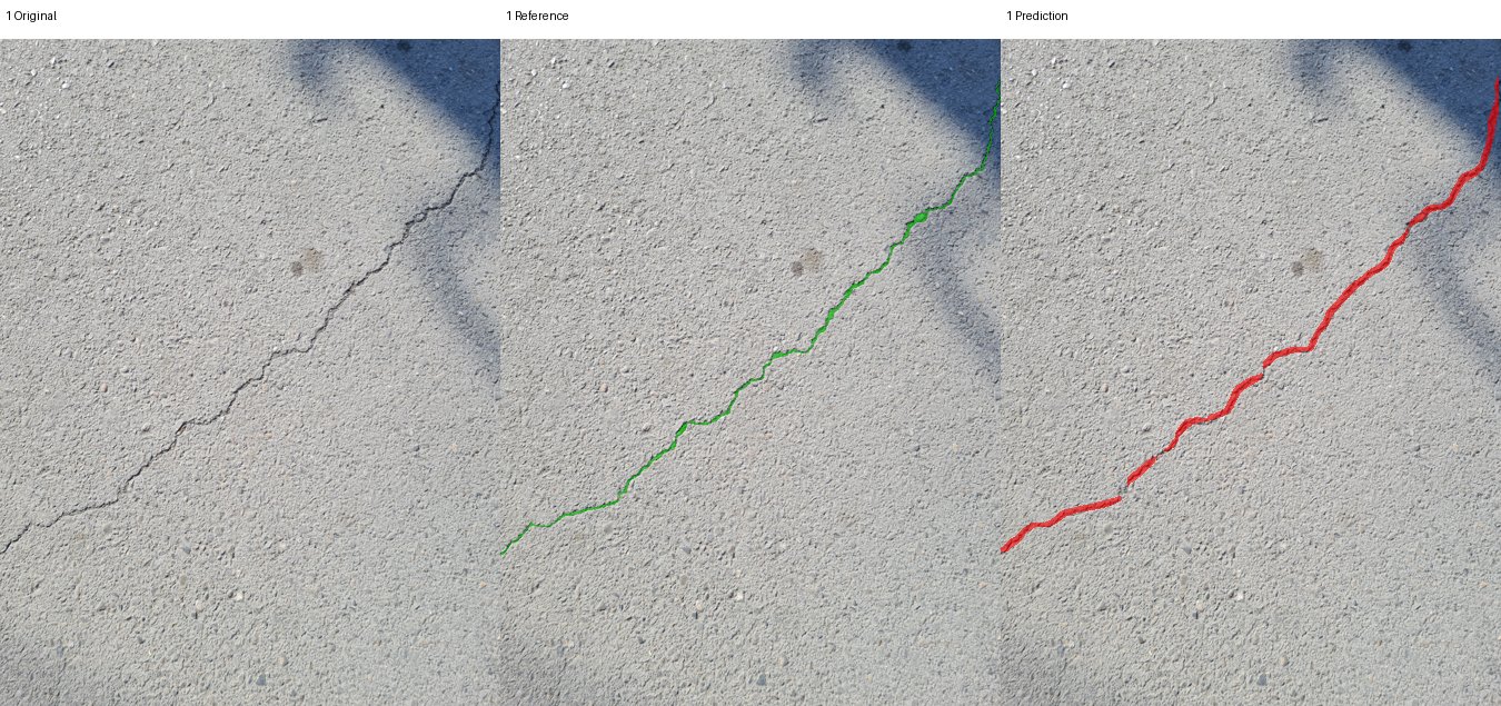 ReferencePrediction
Compare the same image region: green is the dataset reference and red is the saved prediction. Look for changes in thickness and gaps along the trace.
- Checkpoint
- YOLOv8n · OpenSistemas
- Input
- Grayscale + CLAHE
- Overlap IoU
- 0.312 for this image
sut_yolov8n_smoke, image 1.Then, turn the mask into a path
A mask is an area. For length, we need a path through that area. We remove small connected components, skeletonize the remaining regions, split the skeleton at junctions, and discard short branches. Nearby fragments may then be linked when their endpoint distance and orientations satisfy the configured thresholds.
The current settings include a 200-pixel component-area threshold, an 8-pixel branch threshold, and linking within 25 pixels and 25 degrees, with an additional alignment check. These are implementation settings at the evaluated image resolution. They are not physical constants that should be copied unchanged to every camera setup. For an ordered path, length is the sum of the distances between successive pixels:
A horizontal or vertical step contributes one pixel; a diagonal step contributes √2. This follows the trace instead of taking the straight distance between its endpoints. Linking adds a complication. The gap between two fragments was not observed as a continuous crack. The assembled length includes that accepted gap, so we distinguish the two quantities:
Joining fragments can recover a missed section, but it can also connect things that should stay separate. That decision changes the measurement. It belongs in the explanation and the evaluation, not hidden inside a cleanup step.
Orientation and opening width
We use principal component analysis (PCA) to find the direction in which the centreline points are most spread out. The code subtracts their mean, then uses a matrix decomposition to find this main axis. It is an undirected angle: a line at 0 degrees has the same orientation as one at 180 degrees. This is useful for an elongated trace, but it does not describe every local turn or the tangent at a complicated crack tip. Opening width is estimated using the distance transform of the mask. At a skeleton point, twice the distance to the nearest background gives a local width estimate. We record summary statistics rather than pretend the entire crack has one width. That estimate depends on the segmentation boundary and image resolution. It is distinct from W, the width of the structural member. The two “widths” have very different jobs.
Which way do the points spread?
PCA finds the axis along which the centreline points vary most. Rotate the example to see that axis follow the points.
Dominant orientation: 20°
Peach dots: sampled centreline points. Lilac line: the PCA axis through their mean. This is an undirected axis—both ends describe the same orientation. It does not predict where the crack will grow.
Why we added SAM: the member around the crack
The crack detector answers where the crack is. We still need the geometry of the piece of material containing it. In the fracture expression, the ratio changes the geometry factor, so measuring the crack alone leaves an input missing. That is where Segment Anything (SAM) comes in. Its promptable segmentation interface lets us ask for a region using points. We use MobileSAM, which replaces SAM’s heavy image encoder with a lighter encoder while retaining compatibility with the original mask decoder. That made it a practical implementation choice for the prototype; we have not established a deployment speed for our complete pipeline from the model authors’ timings. MobileSAM paper and official implementation. Here, MobileSAM’s job is to delineate the member surface. It is separate from the crack segmentation model. A good crack mask and a good member mask solve different parts of the measurement problem.
Direction first, then the member mask
We first use the dominant orientation from PCA as the axis along which to inspect the member. I use θ for that direction; a remains the model’s crack length, not an angle. Rotating a crack in the image changes this measurement axis. It does not, by itself, establish the loading direction or make an inclined crack compatible with the Mode I benchmark. Prompting directly on the dark trace can select the crack itself. The code therefore takes points along the detected crack and offsets them to either side, perpendicular to its dominant direction. The intended targets are points on the surrounding material. The current implementation uses up to three of the longest detected cracks, with up to three sampled locations on each. It starts with a 12-pixel offset and retries at 25 pixels if the selected mask is too small compared with the crack pixels. Both offsets are image-space heuristics. A point can still land on another object or beyond a narrow member; being generated from a crack does not make it automatically correct.
Follow the direction of the crack
Rotate the trace in the image plane, then follow the measurement. This is a controlled schematic, not a live SAM prediction.
The dominant direction θ defines an axis through the trace. The model's a is a length along a compatible crack, not the angle.
The blue mask covers the complete visible member in this idealized example. A real mask that misses an edge would shorten the measured chord; a mask that leaks into the background could lengthen it. Rotation is in the image plane. The gray dimension is the fixed specimen width W. The gold chord follows the crack direction. They coincide at 0° in this example; at other angles the chord is a CV measurement, not automatically the W of the validated PINN geometry.
Next, a 15 × 15 morphological closing fills narrow holes in the mask so that the crack opening itself does not interrupt the width measurement. Closing can also bridge nearby regions or alter boundaries. We need to inspect the resulting outline rather than assume cleanup always preserves the physical geometry. From a selected point on the crack, the code walks in both directions along its global orientation until it leaves the surface mask. The distance between those intersections is the candidate member extent:
The code names this measurement W_px, but that name does not establish compatibility with the mechanics model. In the validated specimen, W is the plate width along the straight edge-crack axis. If we rotate only the crack inside a fixed rectangle, its inclined boundary-to-boundary chord generally differs from that width. For example, at −8° the demo’s chord crosses the left and right edges and measures about 525.1 pixels, while the horizontal width remains 520 pixels. The sign sets the slope; it does not switch the measurement to the perpendicular dimension. Rotating the entire specimen and its loading together would be a different case. An inclined crack in a fixed specimen needs a compatible fracture model before its chord can be used as W.
The assumptions behind that measurement
There are several conditions we have to keep visible when interpreting this output:
- One relevant member surface. The implementation selects one returned mask and reuses it across the detected cracks. That assumes those cracks belong to the same member. A frame containing several beams or surfaces needs per-member association before applying this procedure.
- The right physical boundaries. The ends of the chord must represent the width boundaries of the chosen edge-crack problem. A paint boundary, shadow, occluder, or texture transition is not necessarily a specimen edge.
- The entire required extent is visible. When the chord reaches the image border, the code flags its width as a lower bound. That flag cannot recover the missing boundary. We should not present it as a fully measured specimen width.
- A compatible crack direction. The global orientation must be meaningful for the approximately straight crack assumed by the backend. A branched or curved network cannot automatically be reduced to this geometry.
- A suitable image-to-length conversion. The mask gives an image-space chord. Using a single scale requires the planar-view assumptions discussed below; segmentation does not correct perspective by itself.
The code also uses a six-pixel boundary-proximity rule to label a crack as edge-connected. That is a candidate classification to verify. A cropped endpoint or an incorrect mask can produce the same signal. Although the prototype contains a centre-crack evaluation path, the manuscript’s PINN validation concerns the single-edge-crack case; those are not interchangeable validation claims. This part of the prototype remains a measurement proposal that needs its own benchmark. The segmentation-to-length experiments later in the post did not validate MobileSAM’s member extent. For a controlled specimen, supplying a known gives us a way to test the mechanics without silently depending on an uncertain surface mask.
Depth, distance, and the front-facing assumption
A 100-pixel trace has no fixed physical length without scale. Surface distance Z is needed only for the depth-based conversion. A known reference or an already calibrated mm/px value supplies scale without Z. One possible source is monocular metric depth: estimating camera-to-surface distance from a single image. Our implementation uses Depth Anything V2 for this step. Its metric checkpoints are important here: relative depth alone does not establish millimetres. The implementation samples positive depths near the crack and takes their median. For a roughly planar surface viewed front-on, distance Z and focal length in pixels give the scale below. Depth Anything V2 metric models.
Here s is millimetres per pixel, L is the physical trace length, and W is the member extent. The focal length must match the image resolution and crop. A calibrated stereo or RGB-D camera can replace the model if its depth is registered to the colour image and expressed in known units; the current file-based adapter accepts depth maps, while a live sensor needs its own adapter. A reference object on the same plane can supply scale directly, without estimating depth. Resizing a depth map is not the same as geometrically registering it.
Which scale source are we actually using?
The backend already implements five ways to obtain millimetres per pixel. They share an output interface, but they do not have the same calibration needs or accuracy. Here is what each route actually does:
| Source in the code | Required input and conversion | Main limitation |
|---|---|---|
| Manual scale | Supply a known mm/px value directly | Valid only for the image geometry in which it was calibrated |
| Reference object | Known physical length divided by its pixel length | Reference and crack must share the relevant plane; endpoint selection adds error |
| Known standoff | Measured surface distance Z divided by calibrated focal length in pixels | Distance and camera angle must be controlled |
| Depth-map file | Load an aligned depth map, convert its units to mm, take median positive depth near the crack, divide by focal length | Registration, invalid returns and sensor depth error; a live camera adapter is still needed |
| Monocular depth (Depth Anything V2 here) | Infer metric depth from RGB, convert metres to mm, sample the same local region and divide by focal length | Learned scale can be biased on unfamiliar scenes; it has not been calibrated against physical specimens in this study |
For example, a reference measuring 50 mm across 200 pixels gives 0.25 mm/px. A 100-pixel trace then measures 25 mm. A depth-based route gives the same scale if Z = 500 mm and focal length = 2000 px. The arithmetic agrees; whether either input is accurate is a separate measurement question. The monocular adapter is implemented, but this is a code inspection, not a new sensor or model validation. The official Depth Anything V2 metric implementation distinguishes metric models from relative-depth models; only the former supplies the units this conversion needs.
The current scalar conversion assumes a front-facing, approximately planar surface. In-plane crack rotation, as in the SAM visual, is fine for illustrating direction; tilting the camera relative to the surface is different. Perspective then changes scale across the image and can distort the measured direction. A calibrated planar view can be rectified, while a nonplanar surface needs a local or 3D treatment. Most importantly, Z is distance to the material surface. It is not the distance a crack penetrates into concrete.
Is there a best distance to use?
There is a tradeoff to measure. Moving closer can give a thin crack more pixels, but can crop out the member boundaries, exceed a sensor’s near range, or make focus difficult. Moving back fits more of the member into the image while giving small features fewer pixels. Stereo depth adds another effect: under a fixed-disparity-error approximation, absolute depth error grows roughly with the square of distance. This is a stereo relationship, not an error law for Depth Anything. The vendor’s depth-quality methodology distinguishes distance accuracy, spatial noise, temporal noise and valid-depth coverage, and its camera guidance notes that accuracy varies with distance.
Here B is stereo baseline and d is disparity in pixels. We have not measured an optimum standoff for this pipeline. The suitable distance depends on the camera, lens, image resolution, lighting and whether the required boundaries fit in frame.
Where the measurement uncertainty comes from
Lighting affects the appearance given to both segmenters. Shadows can create false boundaries; glare, dark regions and motion blur can hide a trace or shift the selected edge. Diffuse lighting, adequate exposure and sharp focus help keep the trace visible. Active and passive depth sensors also respond differently to their environment, so these would be device-specific experiments rather than a universal lighting setting. The existing results do not contain a lighting-versus-distance calibration curve for our full system. MobileSAM contributes uncertainty through the member outline: selecting a neighbouring surface, shrinking the mask, or bridging a gap during closing changes W. An orientation error can make the chord meet a different pair of edges. Separately, a wrong Z or focal length changes the metric scale. To first order:
The terms are signed changes, not a statistical uncertainty bound. Scale affects physical length; an incorrect member boundary also changes the crack-to-width ratio.
Checking the measurements
A convincing overlay is useful for debugging, but it is not enough to establish measurement accuracy. The manuscript’s CV study compares pretrained configurations on 130 SUT-Crack pavement images and 192 MetroDef3D renders. Those renders represent eight geometries under 24 background conditions, so they are not 192 independent crack shapes. The datasets test the segmentation-to-length component; they are not physical replicas of the single-edge-notch mechanics specimen. We evaluated both foreground overlap and assembled-length agreement. Intersection over Union (IoU) measures overlap: the shared mask area divided by the area covered by either mask. The result that matters most for the design is that the model with the best overlap did not consistently have the best length agreement across datasets. It is easy to see how this can happen: a small missing segment or an unwanted connection can change a path substantially, even when most foreground pixels agree. We therefore need to inspect the measurements as well as the masks. We also passed the reference masks through the geometry routine. Those controls still disagreed with the supplied reference lengths, exposing the effects of path construction, calibration, and potentially different length definitions before we even consider predicted masks.
For context, the exploratory raw-RGB YOLOv8n configuration reported mean absolute percentage error (MAPE) in length of 13.35% on SUT-Crack and 4.65% on MetroDef3D in manuscript v14. Those describe agreement with the dataset references. The SUT scale is nominal, the raw-RGB comparison used the same evaluation images, and these results do not establish independently measured physical accuracy for a new inspection scene. Width, orientation, member-surface estimation, and metric depth still need their own quantitative validation. Testing one stage does not automatically validate the complete image-to-mechanics chain.
For dataset files, annotations and documentation, see SUT-Crack on Mendeley Data and MetroDef3D on Zenodo. The numbers above describe our evaluated subsets, not the complete dataset sizes.
Measurement error and mechanics accuracy
CV · Length error against dataset references
Raw-RGB YOLOv8n · mean absolute percentage error · lower is better
These results measure segmentation-to-length agreement. They do not include MobileSAM member-boundary error or physical depth-calibration error.
PINN · Geometry factor against Tada
Prescribed geometry · plane strain · manuscript v14 ratio sweep
The learned factor follows the trend but underpredicts the reference by 5.5–8.1%. Lines connect the five tested ratios; they are not additional test results. Seed spreads are listed in the table below.
How errors travel through the pipeline
| Error source | What it changes | What we should measure |
|---|---|---|
| Missing crack pixels or false bridges | Trace continuity, assembled length and dominant direction | IoU alongside length error, endpoint errors and failure examples |
| Mask too thick or thin | Opening-width estimate; sometimes the skeleton | Width error against independently measured openings |
| MobileSAM misses a member edge or includes background | W and therefore a/W and the geometry factor | Boundary/chord error against known specimen dimensions |
| Depth or focal-length bias | Physical lengths sharing the same scale | Distance bias, repeatability and calibrated mm/px at several standoffs |
| Oblique view, glare or blur | Both segmentation and geometric conversion | Repeat captures with controlled angle, illumination and exposure |
This is why segmentation accuracy alone is not a measurement accuracy. Losing a thin connection can change the centreline length dramatically while affecting few pixels. Depth adds a different error: with focal length fixed, a 10% distance bias gives a 10% physical-length bias. If a and W share exactly that scale, their ratio stays fixed and K changes by the square root of the scale factor—about 4.9% for a 10% increase. If only the member boundary is wrong, the ratio also changes, so that cancellation no longer applies. These are sensitivity examples, not measured error bars for our system.
Where the PINN fits
The mechanics experiment uses prescribed geometry, load and material properties. The PINN combines a smooth neural displacement field with a fixed Williams crack-tip field. The analytical part supplies the square-root displacement behaviour near the tip; the network learns the remaining correction needed to satisfy the specimen boundaries. This builds on Williams’s crack-tip analysis and the equation-residual training idea in Raissi, Perdikaris and Karniadakis.
Here μ is the material’s shear modulus, which describes its resistance to shear deformation. The positive amplitude parameter supplies a direct K readout. A near-tip penalty, called the volumetric cage in the manuscript, discourages the smooth network from absorbing that amplitude. The enrichment is applied globally: multiplying it by a spatial cutoff introduces extra derivative terms into the equilibrium residual. The manuscript also checks K by fitting the Williams displacement field. Agreement between these two extractions is an internal consistency check; agreement with an independent analytical or finite-element reference tests accuracy.
What the PINN recovered against Tada
For the single-edge-crack benchmark, manuscript v14 compares the learned geometry factor with the Tada–Paris–Irwin handbook expression. These are offline mechanics results with prescribed geometry, separate from the CV dataset results above. The table reproduces the manuscript’s plane-strain ratio sweep; ± is seed standard deviation, not an uncertainty interval for a photographed crack.
| Crack ratio a/W | Tada reference F | PINN F, mean ± SD | Absolute error vs Tada |
|---|---|---|---|
| 0.10 | 1.1837 | 1.0874 ± 0.0120 | 8.1% |
| 0.15 | 1.2648 | 1.1743 ± 0.0130 | 7.2% |
| 0.20 | 1.3707 | 1.2817 ± 0.0069 | 6.5% |
| 0.25 | 1.5010 | 1.4094 ± 0.0145 | 6.1% |
| 0.30 | 1.6599 | 1.5685 ± 0.0136 | 5.5% |
The factor increases with crack ratio as expected, but the PINN consistently underpredicts the reference. Low seed variation does not remove that bias. In the manuscript’s separate five-seed reference experiment at a/W = 0.20, plane-strain K was 1013.2 ± 6.6 MPa√mm, compared with 1086.5 analytically and 1083.75 from FEM: 6.7% and 6.5% errors respectively. The manuscript reports slightly different means in its reference-case and ratio-sweep tables; I have kept each with its own reported comparison rather than combining them. Adam-only training was more stable than the tested Adam-plus-L-BFGS schedule for this formulation; this is an experimental finding for these settings, not a general ranking of optimizers.
Across the tested ratios, the PINN captured the increasing geometry factor but retained a consistent underprediction. The CV experiments measured segmentation-to-length agreement separately. These are the two results established in this study; a combined physical camera-to-mechanics accuracy was not measured.
Code and reading
-
MetroDef3D dataset — synthetic crack data and documentation.
-
Williams (1957): On the Stress Distribution at the Base of a Stationary Crack.
-
Tada, Paris and Irwin: The Stress Analysis of Cracks Handbook, third edition.
-
Raissi, Perdikaris and Karniadakis (2019): Physics-informed neural networks.
-
Patnaik et al.: Reduction of Crack Width with Fiber, ACI SP-319.